Forecasting The Aurora: The Art Of Uncertainty

Author: Roisin Martin

For much of my life, I’ve dreamed of seeing the Aurora Borealis. Living in Ireland, a chance to view the Northern Lights is a rare but not impossible occurrence. Every year or so, the media grows abuzz with hope that we might glimpse Nature’s finest light show from our own back gardens. Each time, I stay up all night, head to the darkest field I can find, and pray for clear skies.

Despite this annual ritual, I must admit with some disappointment that I’ve never seen the Northern Lights in person. Sometimes, of course, I can blame the classic Irish weather. Other times, standing under a perfectly clear sky with no trace of green or red, I’ve found myself questioning the accuracy of these forecasts.

This year, I finally decided to investigate why Aurora predictions so often go wrong. I studied both the phenomenon itself and the science of forecasting, in an attempt to understand the reasons behind my annual disappointment. What I found was not just an answer to a personal question, but a window into the limits of prediction in the physical world.

To investigate auroral forecasting, we must first understand the Aurorae themselves. The Aurorae fall under the field of space weather, which is the study of the Sun’s effects on the near Earth environment. Alongside the electromagnetic radiation which provides us with light and heat, the Sun also emits a continuous stream of charged particles, a flow of its own plasma, known as the solar wind. This travels outward at speeds of at least 200 km/s, carrying a magnetic field with it. On top of this, increased solar activity such as coronal mass ejections (CMEs) and solar flares produces strong “gusts” of this wind when huge amounts of matter are flung from the Sun’s surface.

Solar wind interaction with the Earth’s magnetic field

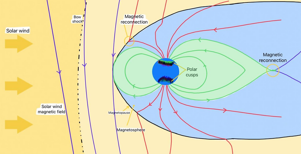
Our Earth also has a magnetic field, generated by the convection currents in its molten core. The region carved out by this field is called the magnetosphere. When the solar wind reaches the boundary of Earth’s magnetosphere, opposing magnetic field lines can snap and reconnect in a process known as magnetic reconnection. The stretched field lines are dragged to the back of the Earth, where they join together again. This allows charged particles from the solar wind to be accelerated along magnetic field lines and into the Earth’s atmosphere at the poles. These particles collide with molecules in our atmosphere, exciting them and causing their electrons to jump to higher energy levels. When these excited molecules return to their ground state, they emit excess energy in the form of light. The resulting light emission is what we observe as the Aurora. 

The color of this light depends on the amount of energy released and the type of molecule. For example, atomic oxygen produces mostly green and some red light, while molecular nitrogen produces blue and purple hues.

Given its spectacular appearance, it is understandable that people want to know when they might see the Aurorae. There are many factors to consider when going “Aurora-hunting.” This includes when it will occur, where it will be visible from and how intense it will be. Many websites offer Aurora forecasts to answer these questions. After visiting a few, it becomes clear that most services rely heavily on a single value: the Kp index.

In short, the Kp index measures the range of disturbance in Earth’s geomagnetic field, compared to calm conditions. This matters because when geomagnetic activity increases, it pushes the auroral oval further from the poles, making displays visible at lower latitudes like Ireland. 

To investigate why auroral forecasts always seem to fail me, I chose to focus solely on the reliability of Kp forecasts. While this is an oversimplification, it is the most widely used tool and still offers a strong baseline for the general public. 

The most prominent Kp forecast is produced by the Space Weather Prediction Centre (SWPC), part of the US National Oceanic and Atmospheric Administration (NOAA) [1]. It is generated using current observations and historical data. On Earth, 13 mid-latitude stations collect ground-based measurements of the magnetic field. In space, the most accurate real-time observations come from spacecraft at the L1 Lagrange point, a point of gravitational equilibrium between the Earth and Sun. One problem with this is that the solar wind only takes 20 to 90 minutes to travel from L1 to Earth, which doesn’t allow much lead time. Furthermore, due to the head-on perspective, it is also difficult to determine the structure of objects travelling directly towards us.

For more advanced notice, other spacecraft take specialized images of the Sun and its corona to gather early information on events like CMEs and coronal holes. However, these images don’t measure the solar wind directly, so forecasts based on them are inherently less reliable.

All of these data are processed through physics-based models, alongside expert interpretation by NOAA forecasters who use their knowledge of past events. The result is a series of forecasts predicting geomagnetic activity, on an adjusted scale from 0 to 9 (0 indicates no deviation from calm conditions), for each 3-hour window over the coming days.

Perhaps the trade-offs in lead time and accuracy are the most obvious difficulties faced when it comes to forecasting Aurorae. The European Space Agency has plans to send a spacecraft to L5 (another point of gravitational equilibrium) to provide another point of reference when observing the solar wind. This mission is called Vigil and is planned to launch in 2031 [2]. This off-angle view would also provide a broader picture of the Sun’s surface, giving advance notice of flares, coronal holes and CMEs.

Not only could this reduce my chances of being let down by an inaccurate forecast, but it could also provide critical warnings to the many industries that operate at the mercy of space weather (think agriculture, aviation, astronaut safety and beyond!)

Another, more abstract difficulty lies not in the limitations of instruments, but in the chaotic nature of the system itself. The magnetosphere satisfies the typical mathematical criteria of a chaotic system. 

Firstly, it is deterministic, its future evolution is entirely determined by its current state, with no randomness involved. If two identical systems began with exactly the same initial conditions, they would evolve identically. However, the magnetosphere is also sensitive to initial conditions. Even the smallest differences between two starting states can grow rapidly, eventually leading to completely different outcomes. 

Lastly, the magnetosphere displays recurrent tendencies. In theory, this means a chaotic system will eventually return arbitrarily close to a previous state, though not in a predictable way. Practically, this is reflected in recurring patterns of geomagnetic activity, even if the exact conditions differ each time.

With a perfect model and infinite knowledge of the initial state, it would be possible to forecast the Earth’s magnetosphere at any future point. In reality, countless obstacles stand in the way and this is just not possible. Collectively, these obstacles are referred to as noise.

There are multiple types of noise. Noise in the measurements is often referred to as observational uncertainty [3]. It is impossible to completely eliminate this, as any real-world measurement made has finite precision. Even with ideal instruments, data can only be recorded to a certain resolution. Past this, small differences will inevitably be lost. Even though the magnetosphere evolves deterministically, the outcomes of two almost-identical states can be drastically different, meaning that even tiny decimal errors like this can have large implications on the final forecast. Of course, we also do not have ideal recording instruments, so the devices themselves contribute a degree of uncertainty too.

Dynamic noise refers to the uncertainties caused by variables not considered by models. The best models do a good job at accounting for the most influential variables, but they still make simplifications and overlook some contributing factors. In the spirit of the famous ‘butterfly’s wings’ analogy, one might imagine that a source of dynamic noise is the inability to track every butterfly’s movement at every moment. It is similarly true of the magnetosphere. While models can process huge amounts of data about some properties like solar wind density or velocity, a vast array of theoretically relevant factors remain unaccounted for. No computers have the ability to do this yet, so simplifications like these are why no model can be truly perfect.

A common approach to managing the sensitivity of chaotic systems is a technique called ensemble forecasting. The “ensemble” is a collection of model-runs, each starting from a slightly altered initial state. The benefit of this method is that it offers a broader scope of possible outcomes. For example, even if we put the most accurate measurements into a magnetospheric model and get a calm forecast, we should still be aware if a model run with small variations predicts magnetic storms. Because we cannot be certain of the initial conditions, it is crucial to consider the array of outcomes that are possible. To Aurora hunters, ensemble forecasts can sometimes seem disappointing, especially when a predicted storm does not happen. But when forecasts err on the side of caution, they’re protecting power grids, satellites, and communications systems. For operators, it is far preferable to suffer the consequences of temporarily shutting down certain systems, rather than risk the costs incurred by an unexpected magnetic storm.

UK Met Office representation of ensemble forecasting in climatology, showing uncertainty growth from initial conditions to long-term predictions. [4]

Armed with information about the trials and tribulations of predicting the Kp index, I wanted to see how these difficulties manifest in actual forecasts. To explore how forecast accuracy changes with geomagnetic activity, I compared official Kp forecasts from the SWPC with the actual values recorded between 22 March and 2 June 2025 [5,6]. I determined how far off each prediction was by examining how well the forecast outperformed a basic average. To contextualise the results, I grouped the real Kp values into three categories: low (0–3), medium (3–6), and high (6–9). This let me investigate whether forecasts were more reliable under calm or stormy space conditions.

It’s generally expected for forecasts to be less accurate the further in advance they are made. This trend is supported by the data from the mid and high-activity forecasts. Notably, for the low-activity forecast, the 1-day lead time appears marginally less accurate. While it could be insignificant, it stands out slightly from the expected pattern. Without further statistical analysis, it’s difficult to say whether this is genuinely anomalous or simply a random fluctuation in the data.

When analyzing the forecast accuracy at different levels of activity, it becomes clear that low-activity conditions can be forecast with some consistency, but more intense geomagnetic events quickly become unpredictable beyond short-term windows. This may be because quiet geomagnetic conditions are primarily influenced by the low-activity solar wind which can be recorded with greater precision, reducing noise in initial measurements. Conversely, increased geomagnetic disturbances are often caused by CMEs and other volatile events. These events introduce more dynamic noise that the model may not consider, thus reducing the accuracy.

This data aligns with the reduced quality of aurora forecasts in Ireland. Because we are situated at a lower latitude, we only experience the Northern Lights when the auroral oval expands outwards, typically during periods of higher geomagnetic activity. Yet, as we have seen, higher Kp forecasts tend to be more unreliable due to the more volatile, less predictable drivers at play. This means that calm nights are easier to forecast than dramatic ones. Unfortunately for Aurora hunters, the most exciting displays tend to be the hardest to pin down in advance.

While the magnetosphere and the atmosphere both behave in complex, chaotic manners, we know that “normal” weather forecasts are generally more accurate than space weather forecasts. This is not because one system is inherently more chaotic. Instead, meteorological forecasting benefits from more data research and public interest. As our society becomes increasingly reliant on infrastructure that is impacted by space weather, we are seeing a push to bring magnetospheric forecasting to the same standard as its more established cousin. Over time, we can expect to see space weather forecasts develop to the same level of accuracy as meteorological ones, and ultimately, the hope is to develop the two fields further as both instrumentation and chaos are further researched.

Investigating auroral forecasting highlights a key difference between physics and maths that is often overlooked. Maths deals with exact quantities. Given initial conditions and enough computing power, you can determine the state of a system at any arbitrary point in the future. Apply this logic to the physical world and everything breaks down. It is crucial to realise that the maths used in physics is only a simplification of what is actually happening. Real properties cannot be truly captured by numbers, and some information is lost in every measurement. Put simply, forecasts are only as good as what we can actually measure, not what we can model. As demonstrated by meteorological forecasting, more data and research can improve accuracy, but they do not solve the underlying problem. Forecasts can’t be perfect. This is not just because we lack information, it’s also because we cannot fully represent the data we do have, let alone account for the countless variables we can’t even begin to measure. 

Despite this, I do believe that auroral forecasts will eventually be accurate enough to guide me to a real display, even if they still fall short of perfection. Some may see these limitations as a failure of science, but that misses the point. They are simply a reminder that Nature is more complex than we can ever truly comprehend. 

Bibliography 

1. NOAA Space Weather Prediction Center. “Planetary K-Index.” Accessed July 14, 2025. https://www.swpc.noaa.gov/products/planetary-k-index

2. European Space Agency. “Vigil.” Accessed July 14, 2025. https://www.esa.int/Space_Safety/Vigil

3. Smith, Leonard. Chaos: A Very Short Introduction. Oxford: Oxford University Press, 2007.

4. Met Office. Ensembles: Forecast Uncertainty Diagram. Accessed July 14, 2025. https://www.metoffice.gov.uk

5. NOAA Space Weather Prediction Center. “3-Day Forecast.” Accessed June 02, 2025. https://www.swpc.noaa.gov/products/3-day-forecast

6. Matzka, J., Stolle, C., Yamazaki, Y., Bronkalla, O., & Morschhauser, A. (2021). The geomagnetic Kp index and derived indices of geomagnetic activity. Space Weather, 19, e2020SW002641. https://doi.org/10.1029/2020SW002641